
Try looking at the picture before naming the mountain. A few black lakes line the upper part of the frame. Below them, grooves in a mountainside converge at a point with a bright lip just to its right. This is Mount Fuji, observed by Europe’s Sentinel-1A around 5:51 a.m. in Japan on 8 December 2024. The oddity is not the absence of colour. The top seems to be in the wrong place. Observation record and data
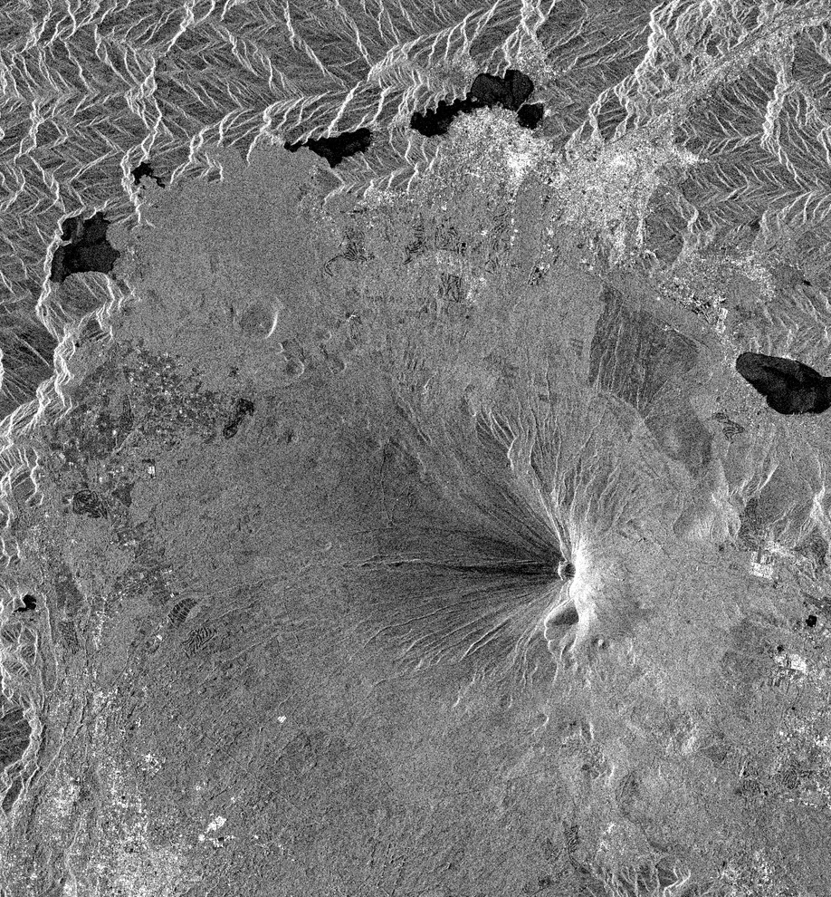
Sentinel-1A, descending orbit, VV polarisation. Brightness represents radar returns transmitted and received in vertical polarisation. North is up and east is right. The acquisition began at 20:51 UTC on 7 December. Contains modified Copernicus Sentinel data (2024). Source observation
Start with the lakes
The second picture is from the optical satellite Sentinel-2B on 2 December. Both views cover the same rectangle, with north at the top. Pick out small Lake Motosu towards the upper left and the pinched outline of Lake Kawaguchi towards the upper right. Their shores fall in roughly the same places in both frames. Now look back at the mountain. The snow reflects light near the summit on the left. In the radar view the grooves appear to meet much farther east. Slide the entire image sideways to make the tops agree and the lakes you just matched will come apart. Sentinel-2B record · Fuji and its lakes on GSI Maps
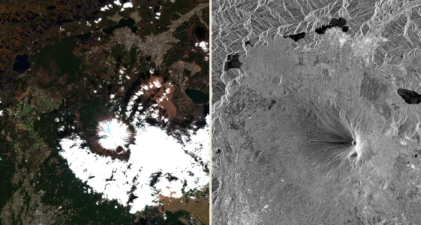
Visible light on 2 December, radar on 8 December, Japan time. Different instruments and dates, matched geographic bounds. Clouds cover part of the southeastern flank in the optical view. Contains modified Copernicus Sentinel data (2024). Optical record · Radar record
Which echo comes home first?
The radar sends its own pulse and times the trip out and back. The instrument looks sideways as the satellite travels along its orbit. On a slope, the order of features in a map view need not be the order of their distances along that oblique line of sight. Geospatial Information Authority of Japan’s explanation · Sentinel-1 products
In the diagram put the sensor S at (0, 6), the foot of the slope A at (4, 0), and a high point B at (5, 2.5). Choose any unit you like. Travelling along the ground you would reach A first. But the straight line from S to A is about 7.21 units long. The line to B is only about 6.10. Double each distance for the return journey and the signal from B still gets back first. To the receiver the peak is nearer. You can reproduce the reversal with a pencil and ruler, without simulating a real satellite orbit.
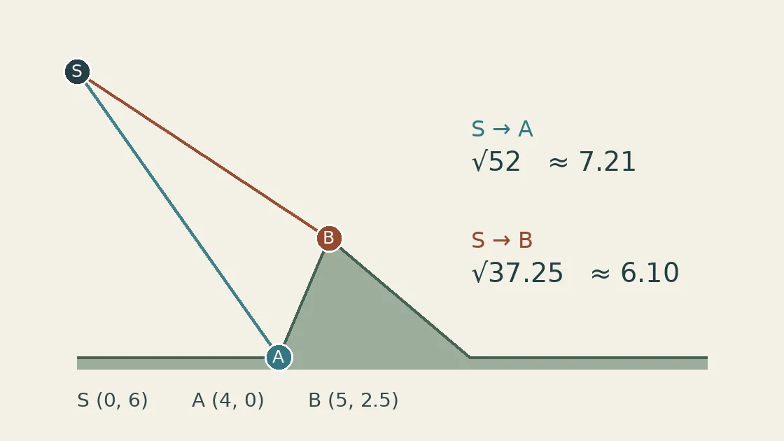
Schematic cross-section in arbitrary units. Doubling each one-way distance preserves the order of the echoes. GSI’s explanation of layover
Where a squeeze becomes a fold
Lower B from 2.5 to 0.5. Its distance from S is now about 7.43, a little longer than the 7.21 to A. The returns bunch together but retain their order. This illustrates the distinction between foreshortening, in which the facing slope appears compressed, and layover, in which the order reverses and returns from distinct locations overlap. Beyond the ridge there may instead be radar shadow, where the signal cannot illuminate the ground. Darkness alone does not identify a shadow. Smooth lake water can also look dark by reflecting energy away from the receiver. Japanese national infrastructure research institute’s Fuji examples, figs. 1.2.3–1.2.5 · Alaska Satellite Facility guide to terrain correction
A 1993 study tested that distinction on Fuji itself. Matsuo compared actual returns with simulations. An ERS-1 view taken 23 degrees off nadir showed layover. A Japanese JERS-1 view taken 35 degrees off nadir showed foreshortening. And in a separate example published by Japan’s infrastructure research institute, the summit appears displaced west. Here it appears east. Change the side from which the satellite looks and the near side changes too. To decide whether actual returns overlap at a particular pixel, the viewing geometry and terrain heights tell us more than a bright streak alone can. Matsuo’s original study and simulations · Institute technical report no. 1110
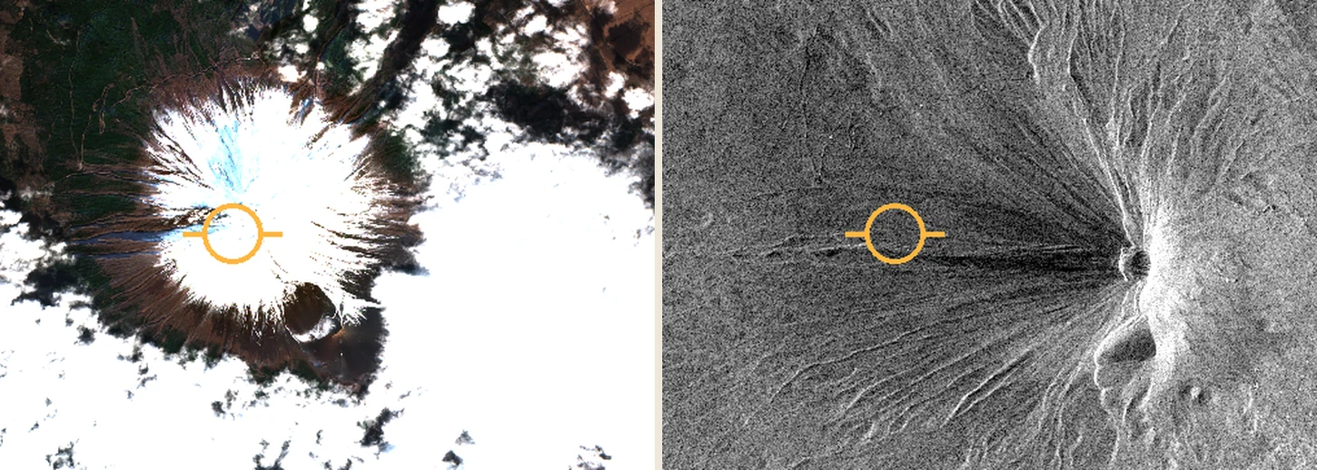
Both circles are centred at 35.3608° N, 138.7275° E. The same crop and marker were applied to both images as a geographic reference. They do not identify a particular rock or radar reflector. Contains modified Copernicus Sentinel data (2024). Reference point on GSI Maps
Why this comparison cannot measure a moving mountain
The optical view comes from a colour composite already registered to a map. For the radar view we interpolated the location grid accompanying a Ground Range Detected (GRD) product to display the returns in the same latitude–longitude frame. We applied no additional terrain correction using a detailed elevation model. The difference visible here arises from relief and the way it was observed and displayed. Measuring the distance from the orange circle to a bright rim would not measure crustal motion. GRD product description · JAXA’s before-and-after comparison in Hokkaido, figures 1 and 3
Go back to the first image once more. The peak still leans, but its peculiar shape now has a history. Before dawn the instrument received a succession of echoes, each arriving at its own moment from a different part of the slope.